Adding Remove and Editing Borders Excel

The Border tab of the Format Cell dialog box provides many options to customize your borders; also, you can use the Formatting toolbar to customize your borders.  

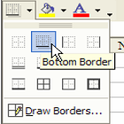
»Applying a Border Style

1- Click on the down arrow beside to the Borders icon on the Formatting toolbar.   

 2- Select the style you want:

»Applying a Border Style

1- Click on the down arrow beside to the Borders icon on the Formatting toolbar.                        2- Select the style you want:

Note: A preview of the pattern is provided in the Sample area.

»Removing Borders

1- Select the cell or range that contains border(s) you want to remove.

2- Click on the down arrow beside to the Borders icon  on the Formatting toolbar.

3- Select the No Border border style from the border menu:

Note: Although a border may appear to be on the left side of a cell, it may actually be on the right side of the adjacent cell. To remove the border, select both cells.

»Changing the Style and Color of Borders

1- Select the cell or range that contains a border style.

2- From the main menu, choose  Format   → Cells →to display the Format Cells dialog

box, and click on the Border tab.

3- Select the location of the border(s) you want from the Border area.

4- Select the style you want from the Line Style area: 

5-Select the color you want from the Line Color drop-down palette:

6-Click OK to apply the border and line style. 

»Using AutoFormat

MS Excel XP has many pre-defined table styles to help you format your table of information quickly. You can apply one of the pre-defined table styles to your table of information.

1- Select a cell inside the table you want to format.

2- From the main menu, choose  Format  →  AutoFormat, select the table style you want, and click OK:

 

»Conditional Formats

To highlight cell values or formula results that you want to monitor, you can identify the

cells by applying conditional formats. For example, suppose a cell contains a value representing the variance between forecast sales and actual sales. Microsoft Excel can apply green shading to the cell if it exceeds or fall short of a certain value.

1- Select the cells you want to format.

2- On the Format menu, click Conditional Formatting.

3- To use values in the selected cells as the formatting criteria, click          Cell Value Is , select

the comparison phrase and then type a value in the appropriate box. 

You can enter a constant value or a formula; you must include an equal sign (=) before the formula.

4- Click Format.

5- Select the font style, font color, underlining, borders, shading, or patterns you want to

Apply .Microsoft Excel applies the selected formats only if the cell value meets the condition.

6-To add another condition, click Add, and then repeat steps         3-5. If you specify multiple

conditions and more than one condition is true, Microsoft Excel applies only the formats

of the first true condition. If none of the specified conditions is true, the cells keep their existing formats.