Formatting Numbers Using the Formatting Toolbar, Excel

You can format your numbers using the Number tab of theFormat Cells dialog box or use the icons on the 

 Formatting toolbar.»Formatting Numbers Using the Formatting ToolbarYou can quickly change the formatting of a cell or range by using the Formatting toolbar.

1- Select the cell or range you want to affect.

2- Choose from the following icons:

Example	Icon
123456 will become $123,456.00 (or your local currency equivalent). Note: This icon may appear as a dollar sign	Currency
18 will become 18%	Percent
456789 will become 456,789.00	Comma
456,789.00 will become 456,789.000	Increase Decimal
456,789.00 will become 456,789.0	Decrease Decimal

 

»Formatting Numbers Using the Format Cells Dialog Box

»Applying the Currency Format

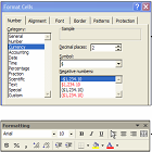
You can further customize your Currency Format with the Format Cells dialog box.

1- From the main menu, choose Format   ──    Cells to display the Format Cells dialog box.

2- Click on the Number tab.

3- Select Currency from the Category scrolling text area:

4-      Select from the following options:

¤ Decimal places: You can adjust the number of decimal places by entering a number

in the spin box or click on the up and down arrows.

¤ Symbol :You can change the currency symbol by selecting the symbol you want from the  dropdown menu.

¤ Negative numbers:You can define how negative numbers appear by selecting one of the options.

5- Click OK to apply the format.

Note: You can preview your formatting in the Sample area.

  »   Applying the Percent Format

You can further customize your Percent Format with the Format Cells dialog box.

1- From the main menu, choose Format   ──    Cells to display the Format Cells dialog box.

2- Click on the Number tab.

3- Select Percentage from the Category scrolling text area.

4- Adjust the number of decimal places by entering a number in the spin box or click on    the up and down arrows:

  

5-Click OK to apply the format.

 

»Applying the Number Format

You can further customize your Number Format with the Format Cells dialog box.

1- From the main menu, choose Format   ──    Cells to display the Format Cells dialog box.

2- Click on the Number tab.

3- Select Number from the Category scrolling text area:

4-Select from the following options:

¤  Decimal places: You can adjust the number of decimal places by entering a number

in the spin box or click on the up and down arrows.

¤  Use 1000 Separator: You can use a comma to separate the thousands.

¤  Negative numbers: You can define how negative numbers appear by selecting one

of the options.

5- Click OK to apply the format.

»Applying Custom Formatting

You can define your own formatting with Custom Formatting.

1- From the main menu, choose Format   ──    Cells to display the Format Cells dialog box.

2- Click on the Number tab.

3- Select Custom from the Category scrolling text area:

4-Select the format that most resembles the one you want (this will display the code in the

Type text box).

5- Edit the code in the Type text box as required.

6- Click OK to apply the format.

»Setting a Fixed Decimal Place for Numeric Values

You can fix the number of decimal places for the values you are entering so that you do not need to enter the decimal point.

1- From the main menu, choose Tools  ──    Options to display the Options dialog box.

2- Click on the Edit tab.

3- Select theFixed Decimal Places check box, enter the number of decimal places you want,    and click OK.

Note: This does not affect data that already exists in the Workbook.